[머신러닝] Chap 5 - Neural Networks

Disclaimer

📣 본 포스트는 조우쯔화의 단단한 머신러닝 책을 요약 정리한 글입니다.

Chap 5. Neural Network

5.1 Neuron Model

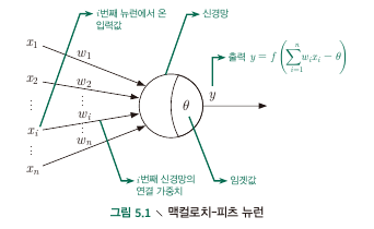
M-P Neuron model

• Input : receive input signals from $n$ neurons
• Process : weighted sum of received signals is compared against the threshold
• Output : signal produced by activation function i.e.) $\text{output = } f({\bf w^T x + b})$

Activation function

• Unit step function (양수이면 1, 음수이면 0)
• sigmoid function ($\sigma(x) = \frac{1}{1+e^{-x}}$) : unit step function은 미분불가능성, 불연속성 등의 좋지 않은 조건으로 인해 sigmoid를 사용.
• $(-\infty, +\infty)$의 값을 $[0,1]$로 밀어넣을 수 있으므로 squashing function이라 불리기도 한다.

5.2 Perceptron and Multi-layer Networks

• Perceptron : 2개 layer (input, output)으로 구성, input layer는 input을 받아서 output layer에 전달, output layer는 M-P neuron으로 threshold 연산 수행.

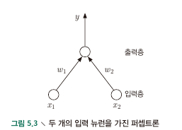
• Perceptron으로 Logic Gate를 구현 가능 (AND, OR, NAND) : by tuning $w_1, w_2, \theta$
• Activation function을 USF로 가정하면,
• AND : $w_1, w_2 = 1, \theta = 2$ : if $x_1, x_2$ are all 1, then output is 1
• OR : $w_1 = 1, w_2 = 1, \theta = 0.5$: if one of $x_1, x_2$$is 1, then output is 1
• NOT : $w_1 = -0.6, w_2 = 0, \theta = -0.5$ : if $x_1$ is 1, then output is 0, else otherwise

Perceptron learning

• weight $w_i$ and threshold $\theta$ can be learned from training data
• threshold를 상수에 대한 weight로 보면 모든 learning process를 weight에 대한 update로 생각할 수 있음.

\[\begin{aligned} w_i &\leftarrow w_i + \Delta w_i \\ \Delta w_i &= \eta (y-\hat y) x_i \\ \eta \in (0,1) &\text{: Learning rate} \end{aligned}\]

• (Single layer) Perceptron은 Linearly seperable problem에 대한 학습만이 가능. if XOR (00, 11 = 0, 01,11=1) 같은 회로는 하나의 선으로 분류가 불가능하므로 학습이 안됨 (but it is guaranteed to converge for linear seperable ploblems)
• 제한적 학습 능력

Multi-layer perceptrons

• Hidden layer : Activation function이 적용되는 input layer와 output layer 사이의 layer.
• Linear seperable problem이 아닌 경우에도 문제 해결이 가능.

5.3 Error Backpropagation Algorithm

• BP (error Back Propagation)
• Constraints(Datas)

\[\begin{aligned} \text{Given dataset } D &= \{({\bf x_i}, y_i)\}, {\bf x_i}\in R^d, y_i \in R^l\ (i=1,2,\cdots, m) \\ \theta_j &\text{ : threshold of the jth output neuron} \\ \gamma_h &\text{ : threshold of the hth hidden neuron} \\ v_{ih} &\text{ : connection weight btw input - hidden} \\ w_{hj} &\text{ : connection weight btw hidden - output} \end{aligned}\]

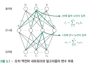
• Consider a single sample $\bf x_i$ to be trained at Multi-layered network with 1 hidden layer
• Hidden Layer의 output $b_i$ :

\[\begin{aligned} b_i &= f(\alpha_h - \gamma_h) \\ \alpha_h &= \sum_{i=1}^d v_{ih} x_i \end{aligned}\]

• Ouptut layer의 output $\hat y_j^k$ :

\[\begin{aligned} \hat y_j ^k &= f(\beta_j -\theta_j) \\ \beta_j &= \sum_{i=1}^q w_{hj}b_h\end{aligned}\]

• Data index $k$, ($\bf x_k$) 에 대한 sum of squared(?) error :

\[E_k = \frac{1}{2} \sum_{j=1}^l (\hat y_j^k - y_j^k)^2\]

• Parameters to tune : $v_{ih}, w_{hj}, \theta_j, \gamma_h$
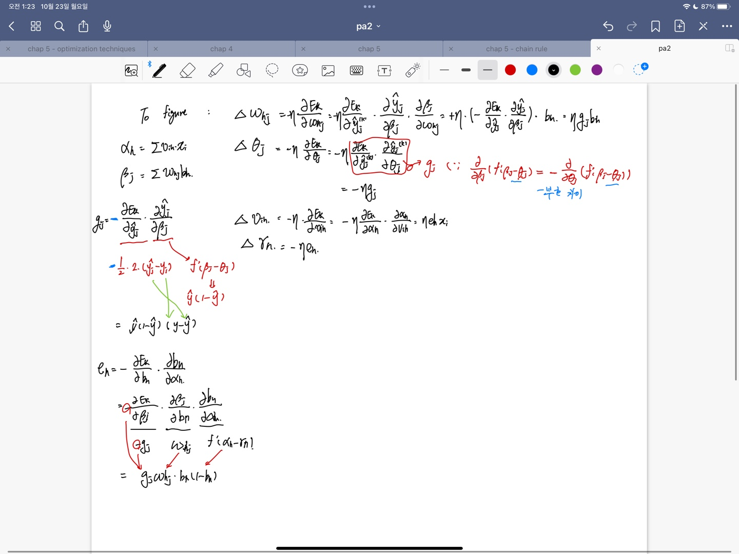
• How to tune : update $v$ with delta v

\[\Delta w_hj = -\eta \frac{\partial E_k}{\partial w_hj}\]

• 각 변수에 대한 Delta는 $E_k$를 object function으로 보고 $E_k$를 내가 tune 하고자 하는 변수에 대한 편미분을 한 다음 학습률 $\eta$와 -1을 곱한 값으로 Delta를 정하여 업데이트 한다. (기울기는 증가하는 방향이 아니라 줄어드는 방향쪽으로 찾아야 Minimum을 찾으니까 -를 붙임.) 이 때 계산은 계산 순서에 따라 chain rule을 적용,
• object function에는 sigmoid function을 사용했다고 가정. $\hat y_j^k$나, hidden layer의 output을 미분할 때에는 weighted sum이 아닌, function안에 weighted sum이 들어간 형태를 사용하게 되므로 function 자체의 derivative를 취해주는 과정, 속미분 과정 잊지말아야.
• Derivation process

Accumulated BP Algorithm

• minimizes the accumulated error on the whole training set

\[E = \frac{1}{m} \sum_{k=1}^m E_k\]

• Tunes parameter less frequently.
• 은닉층 뉴런 개수는 trial-and-error밖에 없음

How to overcome OVERFITTING

• Early stopping : training error 감소, validation error 증가하는 순간 terminate
• Regularization : recall tikhonov regulatization (also minimizes the squared sum of weights)

5.4 Global / Local minimum

• find $\bf w^\ast, \theta^\ast$ s.t. gradient of E is zero : local minimum
• 항상 local minimum이 1개(local=global)임이 보장되지는 않음

How to “jump out” from the local minimum

• Simulated annealing (담금질 기법) : 일정활률로 현재 해보다 나쁜 결과로 이동. (차선의 해를 받을 확률이 점점 줄어들게 되면서, 시간에 따라 algorithm이 안정)
• Stochastic gradient descent : 기울기 계산시 랜덤요소를 추가하여, local minimum에서 계산값이 0이 아닐 수도 있음.
• Genetic algorithm : 비슷..

5.5 Other common neural networks

• NOT considered in this lecture

5.6 Deep learning

• NOT considered in this lecture