[머신러닝] Chap 3 - 리니어 모델

Disclaimer

📣 본 포스트는 조우쯔화의 단단한 머신러닝 책을 요약 정리한 글입니다.

Chap 3. Linear Model

3.1 기본 형식

• d개의 속성을 가진 샘플 $x=(x_1, x_2, x_3, \cdots , x_d)$

\[f({\bf x}) = w_1x_1 + w_2x_2 + \cdots + w_dx_d + b \\ f({\bf x}) = {\bf w^T x }+ b\]

• 학습을 통해 w와 b를 결정. (계수 결정)

3.2 Linear regression

• eg) 하나의 property만을 가진 Data set D를 고려하자

\[\text{consider } D = \{(x_1, y_1), \cdots, (x_m,y_m)\}\]

• Linear regression aims to learn the function:

\[\begin{aligned}f(x) =& wx+b, \ \text{s.t. } f(x_i)\approx y_i \ (i=1\cdots m)\\ ( w^*, b^*) =& argmin_{\substack{(w,b)}}\sum_{i=1}^m (f(x_i)-y_i)^2\end{aligned}\]

• Minimize the mean-square error(MSE)

\[\begin{aligned}&E_{(w,b)} = \sum_{i=1}^m (y_i-wx_i-b)^2\\ &\frac{\partial E_{(w,b)}}{\partial w}=2\bigg(w\sum_{i=1}^m x_i^2-\sum_{i=1}^m(y_i-b)x_i\bigg)\\ &\frac{\partial E_{(w,b)}}{\partial b}= 2\bigg(mb-\sum_{i=1}^m(y_i-wx_i)\bigg)\\ \therefore \ &w = \frac{\sum_{i=1}^m y_i(x_i-\bar x)}{\sum_{i=1}^m x_i^2-\frac{1}{m}\bigg(\sum_{i=1}^m x_i\bigg)^2} \\ &b = \frac{1}{m}\sum_{i=1}^m(y_i-wx_i)\end{aligned}\]

• Multivariate (${\bf x} = (x_1, x_2, \cdots, x_d)$)
• Dataset을 matrix form으로 나타내 보자

\[X = \begin{pmatrix} x_{11} & x_{12} & \cdots & x_{1d} & 1 \\ x_{21} & x_{22} & \cdots & x_{2d} & 1 \\ \vdots & \vdots & \ddots & \vdots & \vdots \\ x_{m1} & x_{m2} & \cdots & x_{md} & 1 \end{pmatrix} = \begin{pmatrix} x_1^T & 1 \\ x_2^T & 1 \\ \vdots & \vdots\\ x_m^T & 1 \end{pmatrix}\] \[\hat{\bf w}^* = argmin_{\hat{\bf w}} ({\bf y - X\hat w^T})({\bf y - X\hat w})\] \[\frac{\partial E_{\hat{\bf w}}}{\partial {\hat{\bf w}}}= 2{\bf X^T(X\hat w - y)}\]

• The solution of multivariate problem

\[\begin{aligned} \text{when }\hat{\bf w} =& \ ({\bf w};b)\\ {\bf \hat{w}^*} =& \ {\bf (X^T X)^{-1}X^T y} \\ f({\bf \hat{x_i}})=& \ {\bf \hat{x_i}}^T {\bf (X^T X)^{-1} X^T y}\end{aligned}\]

• Log linear regression (special case of generalized linear models)
  • Data가 지수 척도에서 변화한다면 사용

\[\begin{aligned}\ln y =& \ {\bf w^T x}+ b \\ y =& \ g^{-1}({\bf w^T x + b})\end{aligned}\]

• for generalized linear models, $g(\cdot )$ is monotonic differentible function (link function)
• $g(\cdot) = \ln(\cdot)$

3.3 Logistic Regression

Binary Classification

• Linear model을 사용하는데, ground truth가 ${0,1}$인 경우
• $z = {\bf w^T x }+ b \in R$ 이므로, 연결해줄 link function을 찾아야 함.
• Unit-step function(Heaviside function)

\[u(z) = \begin{cases} 0, & z<0;\\ 1/2, & z=0;\\1, & z>0\end{cases}\]

• Unit step function은 link function으로 활용할 수 없음 (미분불가능한점이 존재하여 $g^{-1}$이 정의되지 않으므로)
• Sigmoid function

\[y=\frac{1}{1+e^{-x}}\]

• sigmoid function은 differentible하고 monotoic하므로, 이를 변환시켜주면,

\[\ln{\frac{y}{1-y}}= {\bf w^T x }+ b\]

• $y$ : $x>0$일 가능성, $1-y$ : $x<0$일 가능성으로, ln 항에서 둘을 비교하는 것으로 볼 수 있음. 이러한 분수를 odds라고 부름

\[\text{odds} := \frac{y}{1-y}\]

• odds에 로그를 취한 것을 logit이라 부름

\[\text{logit} := \ln{\frac{y}{1-y}}\]

applying maximum likelihood

• logits can be rewritten as

\[\begin{aligned}\ln{\frac{p(y=1\vert {\bf x})}{p(y=0\vert {\bf x})}} =& \ {\bf w^T x }+ b \\ p(y=1\vert {\bf x}) =& \ \frac{e^{w^Tx+b}}{1+e^{w^T x + b}} \\ p(y=0\vert {\bf x}) =& \ \frac{1}{1+e^{w^T x + b}} \end{aligned}\]

• Maximum likelihood method를 통해 $w, b$를 추측하면,

\[l({\bf w}, b) = \sum_{i=1}^m \ln {p(y_i \vert {\bf x_i}; {\bf w}, b)}\]

• 이 때 $\beta = ({\bf w};b), \hat{\bf x} = ({\bf x}; 1)$ 로 가정,

\[l({\bf w}, b) = \sum_{i=1}^m \ln{y_ip_1(\hat {\bf x_i};\beta)+ (1-y_i)p_0(\hat {\bf x_i};\beta)}\] \[l({\bf \beta}) = \sum_{i=1}^m \bigg(-y_i{\bf \beta^T}\hat{\bf x_i} + \ln{\big(1+e^{{\bf \beta^T}\hat{\bf x_i}}\big)}\bigg)\]

• find beta with gradient descent, Newton method

\[{\bf \beta^*} = argmin_{\beta} \ l(\beta)\]

• eg) Newton’s Method,

\[\begin{aligned}{\bf \beta}^{t+1} =& \ {\bf \beta}^t - \bigg(\frac{\partial^2 l(\beta)}{\partial \beta\partial \beta^T}\bigg) \frac{\partial l(\beta)}{\partial \beta} \\ \frac{\partial l(\beta)}{\partial \beta} =& \ \sum_{i=1}^m \hat{\bf x_i} (y_i-p_1(\hat{\bf x_i};{\bf \beta})) \\ \bigg(\frac{\partial^2 l(\beta)}{\partial \beta\partial \beta^T}\bigg) =& \ \sum_{i=1}^m \hat{\bf x_i}\hat{\bf x_i}^T p_1(\hat{\bf x_i};{\bf \beta}) (1-p_1(\hat{\bf x_i};{\bf \beta})) \end{aligned}\]

3.4 Linear Discriminant Analysis (LDA)

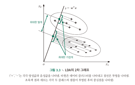
• Data points를 $y=wx+b$에 투영시키고, 같은 label을 가진 점들의 위치가 최대한 가깝도록 $w$와 $b$를 찾는 방법
• 즉 data set이 given일 때 최대화시키는 $y=wx+b$를 찾는 것
• Some variables ($n$ : number of features, $m_i$ : number of data)
  • sample set of the ith class $X_i$ ($n\times m_i$)
  • mean vector of the ith class $ {\bf \mu_i}$ ($n \times 1$)
  • covariance matrix of the i-th class {$\bf \Sigma_i$} ($n \times n$) (각각의 변수들에 대한 공분산을 matrix 형태로 표시)
• After projection to a line
  • the centers of those two classes samples ${\bf w}^T{\bf \mu}_0$, ${\bf w}^T{\bf \mu}_1$
  • the covariances of the two classes samples ${\bf w}^T{\bf \Sigma}_0{\bf w}$, ${\bf w}^T{\bf \Sigma}_1{\bf w}$
• Objective to be maximized

\[J = \frac{\Vert{\bf w^T \mu_0 - w^T \mu_1}\Vert_2^2}{\bf w^T{\bf \Sigma_0}{\bf w}+ \bf w^T{\bf \Sigma_1}{\bf w}}\]

• 분자와 분모로 나누어 생각해보면 분자는 평균의 2-norm, 분모는 co-variance 의 합임을 알 수 있다.

\[J = \frac{ \bf w^T({\bf \mu_0-\mu_1})({\bf \mu_0-\mu_1})^T{\bf w}}{\bf w^T({\bf \Sigma_0 +\Sigma_1}){\bf w}}\]

• The within-class scatter matrix

\[\begin{aligned}{\bf S_w} =& \ {\bf \Sigma_0 + \Sigma_1} \\ =& \ \sum_{{\bf x}\in X_0}({\bf x-\mu_0})({\bf x-\mu_0})^T \\ +& \ \sum_{{\bf x}\in X_1}({\bf x-\mu_1})({\bf x-\mu_1})^T\end{aligned}\]

• Between-class scatter matrix

\[{\bf S_b} =({\bf \mu_0-\mu_1})({\bf \mu_0-\mu_1})^T\]

• Generalized Rayleigh quotient

\[J = \frac{\bf w^T S_b w}{\bf w^T S_w w}\]

• ${\bf w^T S_w w} = 1$이라 하면, maximizing generalized Reyleigh quotient is equivalent to

\[\begin{aligned}min_w -{\bf w^T S_b w} \\ \text{s.t.} {\bf w^T S_w w}=1 \end{aligned}\]

• Using the method of Lagrange multipliers (저런 constraint 문제를 푸는 방법 : lagrangian multiplier)

\[{\bf S_b w} = \lambda {\bf S_w w}\]

• recap the definition of Between class scatter matrix

\[{\bf S_b w} = \lambda ({\bf \mu_0-\mu_1})\]

• 위 두 식을 연립하면,

\[{\bf w} = {\bf S_w^{-1}} ({\bf \mu_0-\mu_1})\]

• Solve by singular value decomposition : ${\bf S_w} = {\bf U\Sigma V^T}$

Extend LDA to multiclass classification problems

• The global scatter matrix

\[\begin{aligned}{\bf S_t} =& \ {\bf S_b} + {\bf S_w} \\ =& \ \sum_{i=1}^m ({\bf x_i-\mu})({\bf x_i-\mu})^T \end{aligned}\]

• Decomposition of within-class scatter matrix

\[\begin{aligned}{\bf S_w} =& \sum_{i=1}^N {\bf S_{w_i}}\\ \text{where } \ S_{w_i} =& \sum_{{\bf x}\in X_i} ({\bf x-\mu_i})({\bf x-\mu_i})^T \\ {\bf S_b} = \ {\bf S_t}-{\bf S_w} =& \sum_{i=1}^N m_i ({\bf \mu_i-\mu})({\bf \mu_i-\mu})^T\end{aligned}\]

• Think about the formula $Var(X) = E(X^2)-E(X)^2$
• Objective :

\[\begin{aligned}\max_{\bf W}\ \ \frac{tr\bigg({\bf W^T S_b W}\bigg)}{tr\bigg({\bf W^T S_w W}\bigg)} \\ \text{where }{\bf W}\in {\bf R}^{d\times (N-1)} \end{aligned}\]

• (trace?) : 각각에 대한 w vector들은 서로서로끼리만 곱해져야하므로 관심있는 항은 diagonal임. 여기서의 $d$ : $n$ (number of features), $N$ : number of classes
• which leads to lagrange multiplier problem

\[{\bf S_B W} = \lambda {\bf S_w W}\]

• $W$ corresponds to d’ largest non-zero eigenvalues of ${\bf S_w^{-1} S_b}$ (d’개의 non-zero eigenvalues로부터 구한 eigenvector를 concat한 게 W이다?) where $d’\leq N-1$

3.5 Multiclass Classification

• N개 클래스를 분류하는 분해법. Binary classification의 확장으로, 3가지 정도의 전형적 분해 전략이 있음
• OvO (One vs. One)
• OvR (One vs. Rest)
• MvM (Many vs. Many)

OvO (One vs One classification)

• N개의 클래스에서 2개씩 선택함. 즉 $_nC_2$개의 Binary classification 문제 생성
• 결괏값의 결정은 가장 많은 선택을 받은 결과를 선택하게 됨.

OvR (One vs Rest classification)

• N개의 클래스 각각을 양성으로, 그 나머지를 음성으로 하여 N개의 classifier 학습.
• 한개만 양성이라면 그 label을, 여러 개가 양성이라면 각 classifier의 예측 신뢰도가 가장 큰 클래스의 레이블을 결과로 선택
• OvO, OvR은 여러 tradeoff가 있지만 결과적으로 성능은 비슷함

MvM (Many vs Many classification)

• N개의 class들을 M번 positive와 negative (혹은 neutral)로 나눔.
• base codeword를 계산.

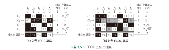
• column에 각 classifier들을, row에 class label을 배치하고 해당 classifier를 train시 어떤 positive,negative value를 사용했는지를 기입한다.
• 생성된 M개의 classifier들을 이용하여 test sample을 분류하는데, 각각의 $C_n$들에 대해 distance가 가장 작은 label을 결과값으로 한다. (해밍거리와 유클리드 거리 사용)
• classifier 자체의 오류를 수정하는 error correction ability가 있으므로 (하나의 classifier의 오류 정도는 크게 영향을 미치지 않음) ECOC라 불림.
• 이론상 코드의 길이($M$)이 증가하는 경우, distance 증가할 수록 성능이 좋아짐.
• Ternary : neutral은 해당 class를 classifier가 사용하지 않았다는 것

3.6 Class Imbalance Problem

• balanced class의 경우
  • $\text{odds : }\frac{y}{1-y}>1$ 이면, 양성으로 판별
• unbalanced class의 경우
  • $\frac{y}{1-y}>\frac{m^+}{m^-}$이면 양성으로 판별
• 관측 odds(ratio of positive samples / negative samples)와 비교하는 것이 타당

Rescaling

• 일반적으로 balanced class에 대한 식을 사용해야 하는데, unbalanced의 경우 odds의 비율을 고려해 줘야 하므로,

\[\frac{y'}{1-y'} = \frac{y}{1-y} \times \frac{m^-}{m^+}\]

1. undersampling : negative samples를 선택적으로 제거하여 balanced class로 만드는 방법
2. oversampling : positive samples 수를 늘려서 balanced class로 만드는 방법
3. threshold-moving : 모든 샘플을 그대로 활용하지만, threshold를 바꾸어 (위 식 처럼) 사용하는 방법