[제어공학개론] Lec 12 - State feedback control, State estimator

📢Precaution

본 게시글은 서울대학교 심형보 교수님의 23-2 제어공학개론 수업 내용을 바탕으로 작성되었습니다.

State-Feedback Control

consider Plant $\dot x = Ax+Bu$, $x \in \Re^n$

$r$의 reference가 있고, Controller는 $u=-Kx+r$

이러한 closed loop system을 state-space representation으로 다음과 같이 쓸 수 있다.

\[\begin{aligned} \dot x &= (A-BK)x + Br \\ y &= Cx+Du \end{aligned}\]

controllability canonical form으로 변환시켜 생각해 봤을 때

\[\begin{aligned} \dot z &= \bar A z + \bar B u \\ u &= -Kz \\ \dot z &= (\bar A - \bar B k)z \end{aligned}\]

Last row of equation above

\[\dot z_n = \begin{bmatrix}-a_1-k_1 & -a_2-k_2 & \cdots & -a_n-k_n\end{bmatrix}\]

즉 state에 적절한 gain $K$를 곱한 feedback control은 characteristic polynomial을 바꾸는 효과가 있음.

Ackermann’s Formula

for controllable $A, B$ (given)

\[\Delta(s) = s^n + a_{n-1}s^{n-1} + \cdots + a_0 = (s-\lambda_1) (s-\lambda_2) \cdots (s-\lambda_n)\]

let $\Delta(s)$ be decired C.P with desired roots 사실 s에는 실수(혹은 complex number)가 들어가야 할 것 같지만, $A-Bk$라는 matrix를 잠시 넣을 수 있다고 해보자.

\[\Delta(A-BK) = (A-BK)^n + a_{n-1}(A-BK)^{n-1} + \cdots a_1 (A-BK) + a_0 I = 0\]

=0이 성립하는 이유는 desired c.p로 $\Delta$를 설정하였기 때문에, Cayley-Hamilton theorem에 의해서 성립. B가 포함되지 않은 항들에 대한 summation은 $\Delta(A)$와 같다. 또한 나머지 항들도 모두 $B, AB, \cdots, A^{n-1}B$와 같이 A, B의 controllability matrix에 등장하는 term으로 표현이 가능하다.

\[\Delta (A-BK) = \Delta (A) - \begin{bmatrix}B & AB & \cdots & A^{n-1}B\end{bmatrix}\begin{bmatrix}* \\ * \\ \vdots \\ K\end{bmatrix}\]

$A^{n-1}B$ term은 단 한번, $(A-BK)^{n-1}$에서 등장하며, 이 때의 계수는 $K$이다.

\[\therefore K = \begin{bmatrix}0 & 0 & \cdots & 1\end{bmatrix} \begin{bmatrix}* \\ * \\ \vdots \\ K\end{bmatrix} = \begin{bmatrix}0 & 0 & \cdots & 1\end{bmatrix} C^{-1} \Delta A\]

State-Observer (Estimator)

모종의 이유로 state를 직접 확인할 수 없을 때, $y(t)=Cx+Du$를 통해 $x$를 알아낼 수 있음.

\[\dot {\hat x} = A\hat x + Bu - L (C\hat x +Du-y)\]

System copy + 보정 term

\[\hat x \rightarrow x \text{ as } t\rightarrow \infty\]

state-feedback controller와 함께 적용되는데, 이 때 $u=-Kx$의 $x$를 모르므로, $u=-K\hat x$로 함.

How to construct matrix $L$

\[\begin{aligned} e(t) :=& \hat x(t) - x(t) \\ \dot e(t) =& \dot {\hat x}(t)-\dot x(t) \\ \dot x =& A\hat x + Bu \\ &- L(C\hat x + Du - y) - Ax \\ =& Ae(t) + LCe(t) \\ =& (A-LC)e(t) \end{aligned}\]

$A-LC$의 eigenvector를 잘 설정하는 방법으로, state observer의 $L$을 알아낼 수 있음.

\[\begin{aligned} (A-LC)^T &= A^T-C^TL^T : \text{A-BK form} \\ L &= \text{acker}(A^T, C^T)^T \end{aligned}\]

Output Feedback Controller

기본 principle은 state feedback + state estimtor

\[\begin{aligned} \dot {\hat x} &= A\hat x + Bu-L(\hat y - y) \\ u &= -k\hat x \\ \text{Let} D &= 0 \text{ for simplicity} \end{aligned}\]

now consider Transfer function of Controller

Controller는 $y$를 입력으로 받고, feedback이 적용된 $u$를 출력함.

\[\begin{aligned} \dot {\hat x} &= (A-BK-LC)\hat x + Ly \\ u &= -k\hat x + 0y \\ C(s) &= -K(sI-(A-BK-LC)^{-1})L \end{aligned}\]

Linearization of two cart example

실제 system의 representation은

\[\begin{aligned} \dot x &= Ax+ Bu \\ \text{Let } e(t) &= x(t)-x^T \end{aligned}\]

여기서 $x_T$는 Target state를 의미한다.

\[\dot e = \dot x - 0 = Ax+Bu\] \[\text{Let} \ u = r^* + v\] \[\dot e = Ae+Ax^T + Bu\]

$r^*$ 은 reference input, 혹은 Steady state input

그렇다면,

\[Ax^T+ Br^*=0\] \[\text{if } x^T \text{ is valid state}\]

왜냐하면 $\dot x = Ax^T + Br^* = 0$ in steady-state

\[\text{set } v \equiv -ke = -K(x(t)-x^T)\] \[\dot e = Ax+B(r^*+v) = Ae+Bv\] \[u = r^*+v=-k(x-x^T)=-Kx+Kx^T\]

즉 reference를 제외한 순수한 $x$에 $k$를 곱한 $v$를 new input으로 보고 $A-Bk$를 해결하는 것과 동일해짐. $e$에 대한 원점$=0$인 input이 되며,

$r^*$은 two-cart system에서 평형점에 도달하면 입력을 안줄것이므로 $0$이다.

실제 주어야 하는

\[u = r^*+v=-k(x-x^T)=-Kx+Kx^T\]

즉 bias term처럼 생긴 $Kx^T$를 입력해주어야 한다.

Tracking control

지금까지의 제어 목표는$ \lim\limits_{t\rightarrow \infty} x(t) = 0$

$x^*(t)$ : desired trajectory

\[\lim\limits_{t\rightarrow \infty} ||x(t)-x^*(t)||=0\]

eg) X measurable, 위의 goal을 만족하는 $u$를 찾아야 한다.

먼저 $x^*(t)$ does it make sense?

\[\begin{aligned}\dot x =& Ax+Bu \\ \exists u^* \text{ s.t. }\dot x^* &= Ax^*+Bu^*(t) \end{aligned}\]

그 다음으로 문제를 풀려면, 어떻게 해야할까?

\[\begin{aligned} e(t) &= x(t) - x^*(t) \\ \dot e(t) &= \dot x - \dot x^* = Ae+ B(u-u^*) \\ &= Ae+Bv \\ \text{where } v &= u-u^* = -ke \\ \dot e &= (A-Bk)e \\ \therefore u &= v+u^* = u^*-K(x-x^*) \end{aligned}\]

Desired output -> desired state

$y^(t)$, 즉 desired output는 알 수 있지만 desired state $x^(t)$는 즉각 알 수 없는 경우가 있음. desired output을 통해서 desired state를 어떻게 알아낼 수 있는가.

plant의 상대 차수가 $n$인 경우 : Relative degree = degree of denominator - degree of numerator

다시 말해 분자에 zero가 없는 경우.

\[\begin{aligned}G(s) &= \frac{b}{s^n + a_{n-1}s^{n-1} + \cdots + a_0} \\s^n G(s) &= \frac{s^n b}{s^n + a_{n-1}s^{n-1} + \cdots + a_0} = b + \frac{b_{n-1}s^{n-1} + \cdots + b_0}{s^n + a_{n-1}s^{n-1} + \cdots + a_0}\end{aligned}\]

즉 출력을 $n$번 미분하게 되면, 입력값을 알 수 있음.

우리의 목표는 $y(t)$를 desired $y^*(t)$로 보내는 것.

$y, y’$, 등 $y$의 미분값들을 $x_1$, $x_2$ 등으로 놓아보자.

\[y(t) =: x_1(t)\]

우리의 희망사항은 $y(t) = y^*(t)$

같은 방법으로 계속 정의하자

\[\begin{aligned} y(t) &=: x_1(t) \\ \dot y (t) &=: x_2(t) \\ y^{(n-1)}(t) &=: x_n(t) \\ y^{(n)}(t) &= \dot x_n(t) \\ \end{aligned}\]

그러면,

\[y^{(n)}(t) = \dot x_n(t)\]

위처럼 정의하는 순간, $1\sim n-1$번째까지의 행은 원래의 Controllability canonical form을 따라가게 되고, 어쨌든 $y$로 만든 것도 system을 설명해야하므로 마지막 줄은 필연적으로 원래 system의 C.P를 담고 있어야 함.

\[y^{(n)}(t) = \dot x_n(t) = -a_0 x_1 -a_1 x_2 + \cdots -a_{n-1}x_n +bu\]

즉 이를 만족시키기 위해서는 desired $x$를 다음과 같이 두면 됨.

\[x^{(t)} = [y(t), \ \dot y(t), \ \cdots, \ y^{(n)}(t)]^T\]

또한, 여기서 desired output이 valid한지를 확인하기 위해 마지막 식에 $u^*$를 넣으면,

\[-a_0 x_1^* -a_1 x_2^* + \cdots -a_{n-1}x_n^* +bu^*=y^{(n)}(t)\]

이를 위해서는 desired output은 $n$번 미분 가능한 $C^n$ smooth curve이면서, system의 relative degree는 $n$이어야 함. 만약 system의 relative degree가 $n$이 아니라면, 즉 zero가 존재한다면, $x^*$는 유일하지 않음.

Separation Principle

Output feedback control에서 $K$에 의한 eigenvalue와 $L$에 의한 eigenvalue는 separable하다. 즉, observer를 사용한 경우 state feedback에서 설정한 $K$에서 좋은 위치에 둔 e.v.는 그대로 있음 즉 $K$를 이용해 place한 eigenvalue는 Observer에 의해 바뀌지 않는다

\[\begin{aligned}\dot {\hat x} &= (A - (BK + LC))\hat x + Ly \\u &= -K\hat x\end{aligned}\]

Let’s consider closed loop system, considering real and estimated state ($2n$차 system)

\[\begin{aligned}\dot x &= Ax + Bu = Ax - BK\hat x \\\dot {\hat x} &= (A - BK - LC)\hat x - LCx \\\begin{pmatrix} \dot x \\ \dot {\hat x} \end{pmatrix} &= \begin{pmatrix} A & -BK \\ LC & A - BK - LC \end{pmatrix} \begin{pmatrix} x \\ {\hat x} \end{pmatrix} + \text{No external signal} \\ & \text{multiply matrix :} \begin{bmatrix} I & 0 \\ -I & I \end{bmatrix}\end{aligned}\]

$(x, \hat x) \rightarrow (x ,\hat x - x)$ 의 translation

\[\begin{pmatrix}\dot x \\ \dot {e}\end{pmatrix} = \begin{pmatrix}A-BK & * \\ 0 & A-LC\end{pmatrix}\begin{pmatrix} x \\ e\end{pmatrix}\]

$\dot x$의 eigenvalue는 $K$에 의해 설정된 eigenvalue임을 알 수 있음.

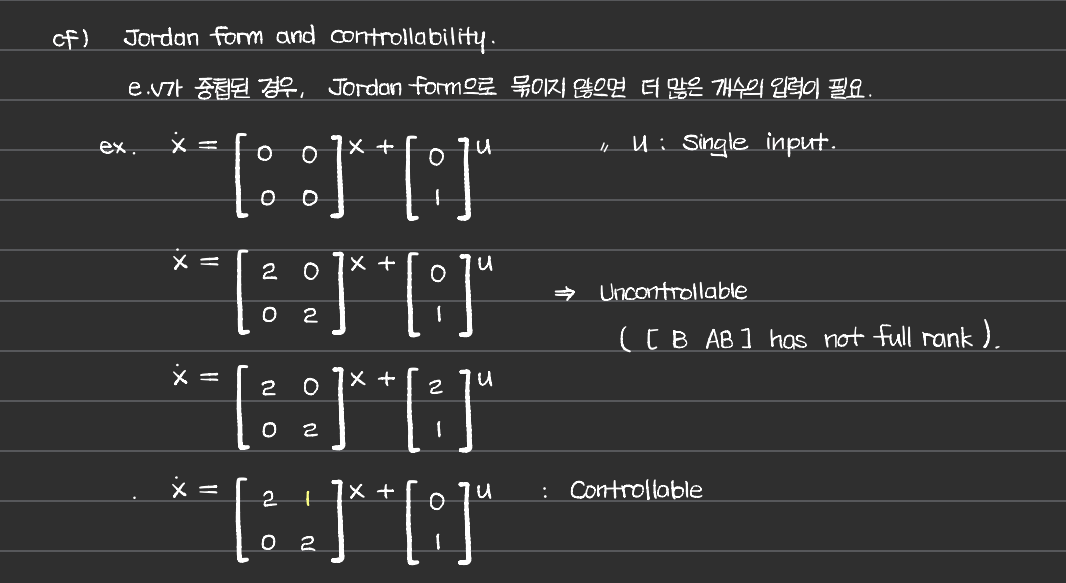
Jordan form and controllability

Jordan form으로 나타냈을 떄 eigenvalue들이 중첩된 경우, Jordan block으로 묶이지 않다면, single input이 아닌 multi input이어야 controllable해짐.