[전선대 Assignment] SIR model, Fractals

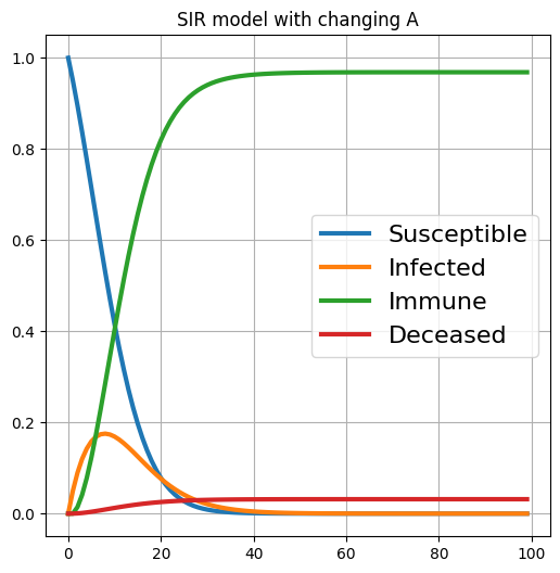
Problem 1 - Simulation of the SIR model

In this problem you will be asked to use python to simulate the SIR model. Let’s define state $x_t$ as the portion of the population that are susceptible, infected, immune, decease to or by the COVID-19 virus at timestep $t$. That is, $x_t$ is a vector of 4 dimensions with values between 0 and 1. The epidemic dynamics matrix $A$ is defined as follows:

1. Among suceptible population:
   • $5\% * (0.99)^t $acquire the disease
   • $95\% * (0.99)^t$ remain susceptible
2. Among infected population:
   • $1\%$ dies
   • $10\%$ recovers with immunity
   • $4\%$ recoveres without immnuity(back to being susceptible)
   • $85\%$ remain infected
3. All immune and dead stay in their states

Please read the comments carefully and fill in the TODO marks

# Import the required libraries
import matplotlib.pyplot as plt
import numpy as np

# The epidemics dynamics matrix A (initial value @t=0)

def Matrix(t): ## return epidemics dynamics matrix A at step t
    A = np.array([
        ################ TODO #####################
        [0.95*(0.99)**t,0.04,0,0],
        [0.05*(0.99)**t,0.85,0,0],
        [1-(0.99)**t,0.1,1,0],
        [0,0.01,0,1]
    ])
    return A

# Set some variables and np array to save the state x
timesteps = 100
x_s = np.zeros((timesteps, 4))
x_s[0] = np.array([1, 0, 0, 0])
# x_s save the state x_t for all timesteps
# Simulate and fill in this array

# We will now start simulating and updating the epidemics array
# Remeber the state x_t should sum up to 1 for every timestep!
# simulate for timesteps - 1 times since we have intial state x_0 = [1, 0, 0, 0]
for step in range(timesteps - 1):
    ################ TODO #####################
    x_s[step+1] = np.matmul(Matrix(step),x_s[step])

# Visualize the state trajectory
fig, ax = plt.subplots(figsize=(6, 6))
label = ['Susceptible', 'Infected', 'Immune', 'Deceased']
for idx in range(len(label)):
    ax.plot(x_s[:, idx], lw=3, label=label[idx])
ax.grid()
ax.legend(fontsize=16)
ax.set_title('SIR model with changing A')
plt.show()

Output:

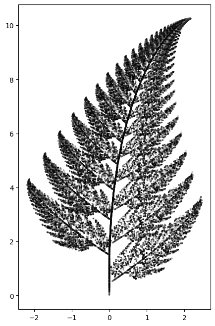
Problem 2 - Fractals

In this problem you will be asked to draw fractals based on linear dynamic systems. Recall from yout classes that when offset is present, the linear dynamics system can be written as

\[x_{t + 1} = A_tx_t + c_t\]

But different to the problem above, we will use more than one dynamics to draw fractals. That is, with the state xt beging the 2D coordinates at time $t$, the state changes with the following probabilities:

1. $x_{t+1} = \begin{bmatrix} 0.86 & 0.03 \ -0.03 & 0.86 \end{bmatrix} + \begin{bmatrix} 0 & 1.5 \end{bmatrix}$, with probablity 0.79
2. $x_{t+1} = \begin{bmatrix} 0.2 & -0.25 \ 0.21 & 0.23 \end{bmatrix} + \begin{bmatrix} 0 & 1.5 \end{bmatrix}$, with probablity 0.11
3. $x_{t+1} = \begin{bmatrix} -0.15 & 0.27 \ 0.25 & 0.26 \end{bmatrix} + \begin{bmatrix} 0 & 0.45 \end{bmatrix}$, with probablity 0.07
4. $x_{t+1} = \begin{bmatrix} 0 & 0 \ 0 & 0.17 \end{bmatrix} + \begin{bmatrix} 0 & 0 \end{bmatrix}$, with probablity 0.03

Please read the comments carefully and fill in the TODO marks

# Let's define A's and C's
A_s = np.array([[[.86, .03],
              [-.03, .86]],
             [[.2, -.25],
              [.21, .23]],
             [[-.15, .27],
              [.25, .26]],
             [[0., 0.],
              [0., .17]]])
c_s = np.array([[[0,1.5]],
             [[0,1.5]],
             [[0,0.45]],
             [[0,0]]])

# Define the number of timesteps to simulate and where to save the trajectory
timesteps = 30000
################ TODO #####################
X = np.zeros((2, timesteps))

# The probablity for each dynamic
################ TODO #####################
prob = np.array([0.79, 0.11, 0.07, 0.03])

# Now let's simulate via python random library
from random import random


for i in range(timesteps - 1):
    ################ TODO #####################
    randnum = random()
    if randnum<prob[0]:
        j=0
    elif randnum<prob[0]+prob[1]:
        j=1
    elif randnum<prob[0]+prob[1]+prob[2]:
        j=2
    else:
        j=3
    X[:,i+1]=np.matmul(A_s[j],X[:,i])+c_s[j]

# Visualization of the trajectory
# Color starts from red to green
colors = np.zeros((timesteps, 3)).astype(np.float32)
for _idx in range(timesteps):
    delta = 1 / timesteps
    R = 1 - (delta * _idx)
    colors[_idx] = np.array([R, R, R])
fig, ax = plt.subplots(figsize = (5,8))
ax.scatter(X[0,:],X[1,:], s=2, c=colors)
plt.show()

Output: